3D Series Chapter 3: Vectors

by Rel (Richard Eric M. Lope)

Vectors are cool!!!

It's almost impossible to do graphics programming without using vectors. Almost all math concerning 3d coding uses vectors. If you hate vectors, read on and you'll probably love them more than your girlfriend after you've finished reading this article. ;*)

What are vectors?

First off, let me define 2 quantities: The scalar and vector quantities. Okay, scalar quantities are just values. One example of it is Temperature. You say, "It's 40 degrees Celsius here", and that's it. No sense of direction. But to define a vector you need a direction or sense. Like when the pilot say's, "We are 40 kilometers north of Midway". So a scalar quantity is just a value while a vector is a value + direction.

Look at the figure below: The arrow (ray) represents a vector. The "head" is its "sense" (direction is not applicable here) and the "tail" is its starting point. The distance from head to tail is called its "magnitude".

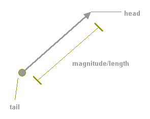
In this vector there are 2 components, the X and Y component. X is the horizontal and Y is the vertical component. Remember that "ALL VECTOR OPERATIONS ARE DONE WITH ITS COMPONENTS."

I like to setup my vectors in this TYPE:

The difference between the "sense" and "direction" is that direction is the line the vector is located while sense can go either way on that line.

Definitions

*|v| means that |v| is the magnitude of v.

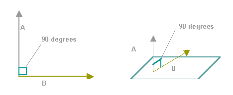
*Orthogonal vectors are vectors perpendicular to each other. It's sticks up 90 degrees.

To get a vector between 2 points:

2d:

3d:

QB code:

where: (x2-x1) is the horizontal component and so on.

Vectors are not limited to the cartesian coordinate system. In polar form:

Resolving a vector by its components

Suppose a vector v has a magnitude 5 and direction given by Theta = 30 degrees. Where theta is the angle the vector makes with the positive x-axis. How do we resolve this vectors' components?

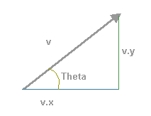
Remember the Polar to Cartesian conversion?

Let vx = horizontal component
Let vy = horizontal component
Let Theta = Be the angle

So...

What I've been showing you is a 2d vector. Making a 3d vector is just adding another component, the Z component.

Operations on vectors needed in 3d engines

Scaling a vector(Scalar multiplication)

Purpose:

This is used to scale a vector by a scalar value. Needed in the scaling of models and changing the velocity of projectiles.

Equation:

v = v * scale


QB code:

v.x = v.x * Scale
v.y = v.y * Scale
v.z = v.z * Scale


Getting the Magnitude(Length) of a vector

Purpose:

Used in "Normalizing"(making it a unit vector) a vector. More on this later.

Equation:

|V| = Sqr(v.x^2 + v.y^2 + v.z^2)


QB code:

Mag! = Sqr(v.x^2 + v.y^2 + v.z^2)


Normalizing a vector

Purpose:

Used in light sourcing, camera transforms, etc. Makes the vector a "unit-vector" that is a vector having a magnitude of 1. Divides the vector by its length.

Equation:

 v = v
-------
  |v|


QB code:

Mag! = Sqr(v.x^2 + v.y^2 + v.z^2)
v.x = v.x / mag!
v.y = v.y / mag!
v.z = v.z / mag!


The DOT Product

Purpose:

Used in many things like lightsourcing and vector projection. Returns the cosine of the angle between any two vectors (Assuming the vectors are Normalized). A Scalar. The dot product is also called the "Scalar" product.

Equation:

v.w = v.x* w.x + v.y* w.y + v.z* w.z


QB code:

Dot! = v.x* w.x + v.y* w.y + v.z* w.z


Fun fact:

* 2 Vectors are orthogonal if their dot product is 0.
Proof: "What is the cosine of 90?"

The CROSS product

Purpose:

Used in lightsourcing, camera transformation, back-face culling, etc. The cross product of 2 vectors returns another vector that is orthogonal to the plane that has the first 2 vectors. Let's say we have vectors U and F.

Equation:

U x F = R


QB code:

R.x = U.y * F.z - F.y * U.z
R.y = U.z * F.x - F.z * U.x
R.z = U.x * F.y - F.x * U.y


Fun facts:

* C is the vector orthogonal to A and B.
* C is the NORMAL to the plane that includes A and B. The cross-product of any two vectors can best be remembered by the CRAMERS RULE on DETERMINANTS. Thought of it while taking a bath. I'll tell you when I finish my matrix chapter.
* The cross product is exclusive to 3d and its also called the "Vector" product.



Vector Projection

Purpose:

Used in resolving the second vector of the camera matrix (Thanks Toshi!). For vectors A and B...



Equation:

U.Z * Z


QB code:

Let N = vector projection of U to Z. The vector parallel to Z.

T! = Vector.Dot(U, Z)

N.x = T! * Z.x
N.y = T! * Z.y
N.z = T! * Z.z


Adding vectors

Purpose:

Used in camera and object movements. Anything that you'd want to move relative to your camera. Adding vectors is just the same as adding their components. Let A and B be vectors in 3d, and C is the sum:

Equations:

C = A + B
C = (ax + bx) + (ay + by) + (az + bz)


QB code:

c.x = a.x + b.x
c.y = a.y + b.y
c.z = a.z + b.z

Now that Most of the Math is out of the way....

Applications

WireFraming and Backface culling

I like to make use of types with my 3d engines. For Polygons:

TYPE Poly
    p1 AS INTEGER
    p2 AS INTEGER
    p3 AS INTEGER
END TYPE


P1 is the first vertex, p2 second and p3 third. Let's say you have a nice rotating cube composed of points, looks spiffy but you want it to be composed of polygons (Triangles) in this case). If we have a cube with vertices:

Vtx1  50, 50, 50  :x,y,z
Vtx2 -50, 50, 50
Vtx3 -50,-50, 50
Vtx4  50,-50, 50
Vtx5  50, 50,-50
Vtx6 -50, 50,-50
Vtx7 -50,-50,-50
Vtx8  50,-50,-50


What we need are connection points that define a face. The one below is a Quadrilateral face (4 points)

Face1 1, 2, 3, 4
Face2 2, 6, 7, 3
Face3 6, 5, 8, 7
Face4 5, 1, 4, 8
Face5 5, 6, 2, 1
Face6 4, 3, 7, 8


Face1 would have vertex 1, 2, and 3 as its connection vertices.

Now since we want triangles instead of quads, we divide each quad into 2 triangles, which would make 12 faces. It's also imperative to arrange your points in counter-clockwise or clockwise order so that backface culling would work. In this case I'm using counter-clockwise.

The following code divide the quads into 2 triangles with vertices arranged in counter-clockise order. Tri(j).idx will be used for sorting.

QB code:

j = 1
FOR i = 1 TO 6
    READ p1, p2, p3, p4  'Reads the face (Quad)
    Tri(j).p1 = p1
    Tri(j).p2 = p2
    Tri(j).p3 = p4
    Tri(j).idx = j
    j = j + 1
    Tri(j).p1 = p2
    Tri(j).p2 = p3
    Tri(j).p3 = p4
    Tri(j).idx = j
    j = j + 1
NEXT i


To render the cube without backface culling, here's the pseudocode:

1. Do
2. Rotatepoints
3. Project points
4. Sort (Not needed for cubes and other simple polyhedrons)
5. Get Triangles' projected coords
     ie.
       x1 = Model(Tri(i).P1).ScreenX
       y1 = Model(Tri(i).P1).ScreenY
       x2 = Model(Tri(i).P2).ScreenX
       y2 = Model(Tri(i).P2).ScreenY
       x3 = Model(Tri(i).P3).ScreenX
       y3 = Model(Tri(i).P3).ScreenY
6. Draw
       Tri x1,y1,x2,y2,x3,y3,color


Backface Culling

Backface culling is also called "hidden face removal". In essense, it's a way to speed up your routines by NOT showing a polygon if it's not facing towards you. But how do we know what face of the polygon is the "right" face? Let's take a CD as an example, there are 2 sides to a particular CD. One side that the data is to be written and the other side where the label is printed. What if we decide that the Label-side should be the right side? How do we do it? Well it turns out that the answer is our well loved NORMAL. :*) But for that to work, we should *sequentially* arrange our vertices in counter or clockwise order.

If you arranged your polys' vertices in counter-clockwise order as most 3d modelers do, you just get the projected z-normal of the poly and check if its greater than(>)0. If it is, then draw triangle. Of course if you arranged the vertices in clockwise order, then the poly is facing us when the Z-normal is <0.

Counter-Clockwise arrangement of vertices:



Clockwise Arrangement of vertices:



Since we only need the z component of the normal to the poly, we could even use the "projected" coords (2d) to get the z component!

QB code:

Znormal = (x2 - x1) * (y1 - Y3) - (y2 - y1) * (x1 - X3)
IF (Znormal > 0) THEN   '>0 so vector facing us
    Drawpoly x1,y1,x2,y2,x3,y3
END IF


Here's the example file:
3dwire.bas

Sorting

There are numerous sorting techniques that I use in my 3d renders here are the most common:

1. Bubble sort (modified)
2. Shell sort
3. Quick sort
4. Blitz sort (PS1 uses this according to Blitz)

I won't go about explaining how the sorting algorithms work. I'm here to discuss how to implement it in your engine. It may not be apparent to you (since you are rotating a simple cube) but you need to sort your polys to make your renders look right. The idea is to draw the farthest polys first and the nearest last. Before we could go about sorting our polys we need a new element in our polytype.

TYPE Poly
    p1 AS INTEGER
    p2 AS INTEGER
    p3 AS INTEGER
    idx AS INTEGER
    zcenter AS INTEGER
END TYPE


*Idx would be the index we use to sort the polys. We sort via IDX, not by subscript.
*Zcenter is the theoretical center of the polygon. It's a 3d coord (x,y,z)

To get the center of any polygon or polyhedra(model),you add all the 3 coordinates and divide it by the number of vertices (In this case 3).

Since we only want to get the z center:

Zcenter = Model(Poly(i).p1)).z + Model(Poly(i).p2)).z + Model(Poly(i).p3)).z
Zcenter = Zcenter / 3


Optimization trick:

We don't really need to find the *real* Zcenter since all the z values that were added are going to be still sorted right. Which means... No divide!!!

Now you sort the polys like this:

FOR i% = LBOUND(Poly) TO UBOUND(Poly)
    Poly(i%).zcenter = Model(Poly(i%).p1).Zr + Model(Poly(i%).p2).Zr + Model(Poly(i%).p3).Zr
    Poly(i%).idx = i%
NEXT i%

Shellsort Poly(), Lbound(Poly), UBOUND(Poly)


To Draw the model, you use the index(Poly.idx)

FOR i = 1 TO UBOUND(Poly)
    j = Poly(i).idx
    x1 = Model(Poly(j).p1).scrx  'Get triangles from "projected"
    x2 = Model(Poly(j).p2).scrx  'X and Y coords since Znormal
    x3 = Model(Poly(j).p3).scrx  'Does not require a Z coord
    y1 = Model(Poly(j).p1).scry
    y2 = Model(Poly(j).p2).scry
    y3 = Model(Poly(j).p3).scry

        'Use the Znormal,the Ray perpendicular(Orthogonal) to the
        'Screen defined by the Triangle (X1,Y1,X2,Y2,X3,Y3)
        'if Less(>) 0 then its facing in the opposite direction so
        'don't plot. If <0 then its facing towards you so Plot.

    Znormal = (x2 - x1) * (y1 - y3) - (y2 - y1) * (x1 - x3)
    IF Znormal < 0 THEN
        DrawTri x1, y1, x2, y2, x3, y3
    END IF
NEXT i


Here's a working example:
sorting.bas

Spherical and cylindrical coordinate systems

These 2 systems are extentions of the polar coordinate system. Where polar is 2d these 2 are 3d. :*)

Cylindrical coordinate system

The cylindrical coodinate system is useful if you want to generate models mathematically. Some examples are Helixis, Cylinders (of course), tunnels or any tube-like model. This system works much like 2d, but with an added z component that doesn't need and angle. Here's the equations to convert cylindrical to rectangular coordinate system.

Here's the Cylindrical to rectangular coordinate conversion equations. Almost like 2d. Of course this cylinder will coil on the z axis. To test yourself, why dont you change the equations to coil it on the y axis?

x = COS(theta)
y = SIN(theta)
z = z


To generate a cylinder:

i = 0
z! = zdist * Slices / 2
FOR Slice = 0 TO Slices - 1
    FOR Band = 0 TO Bands - 1
        Theta! = (2 * PI / Bands) * Band
        Model(i).x = radius * COS(Theta!)
        Model(i).y = radius * SIN(Theta!)
        Model(i).z = -z!
        i = i + 1
    NEXT Band
    z! = z! - zdist
NEXT Slice


Here's a 9 liner I made using that equation.
9liner.bas

Spherical coordinate system

This is another useful system. It can be used for Torus and Sphere generation. Here's the conversion:

x = SIN(Phi)* COS(theta)
y = SIN(Phi)* SIN(theta)
z = COS(Phi)


Where: Theta = Azimuth; Phi = Elevation

To generate a sphere:

i = 0
FOR SliceLoop = 0 TO Slices - 1
    Phi! = PI / Slices * SliceLoop
    FOR BandLoop = 0 TO Bands - 1
        Theta! = 2 * -PI / Bands * BandLoop
        Model(i).x = -INT(radius * SIN(Phi!) * COS(Theta!))
        Model(i).y = -INT(radius * SIN(Phi!) * SIN(Theta!))
        Model(i).z = -INT(radius * COS(Phi!))
        i = i + 1
    NEXT BandLoop
NEXT SliceLoop


Here's a little particle engine using the spherical coordinate system.
fountain.bas

Here's an example file to generate models using those equations:
gen3d.bas

Different Polygon fillers

Flat Filler

Tired of just wireframe and pixels? After making a wireframe demo, you'd want your objects to be solid. The first type of fill that I'll be introducing is a flat triangle filler. What?! But I could use PAINT to do that! Well, you still have to understand how the flat filler works because the gouraud and texture filler will be based on it. ;*)

Now how do we make a flat filler? Let me introduce you first to the idea of LINEAR INTERPOLATION. How does interpolation work?

Let's say you want to make dot on the screen at location (x1,y1) to (x2,y2) in 10 steps?

Let A = (x1,y1)
B = (x2,y2)
Steps = 10

f(x) = (B-A)/Steps


So....

dx! = (x2-x1)/steps
dy! = (y2-y1)/Steps

x! = x1
y! = y1
FOR a = 0 TO steps - 1
    PSET (x,y), 15
    x! = x! + dx!
    y! = y! + dy!
NEXT a


That's all to there is to interpolation. :*)

Now that we have an idea of what linear interpolation is we could make a flat triangle filler.

The 3 types of triangles

1. Flat Filled

   1. Flat Bottom

      

   2. Flat Top

      

   3. Generic Triangle

      

   In both the Flat Top and Flat bottom cases, it's easy to do both triangles as we only need to interpolate A to B and A to C in Y steps. We draw a horizontal line in between (x1,y) and (x2,y).

   The problem lies when we want to draw a generic triangle since we don't know if it's a flat top or flat bottom. But it turns out that there is an all too easy way to get around with this. Analyzing the generic triangle, we could just divide the triangle into 2 triangles. One Flat Bottom and One Flat Top!

   We draw it with 2 loops. The first loop is to draw the Flat Bottom and the second loop is for the Flat Top.

   

   Pseudo Code:

   TOP PART ONLY!!!! (FLAT BOTTOM)

   1. Interpolate a.x and draw each scanline from a.x to b.x in (b.y-a.y) steps.

      ie. a.x = x3 - x1
          b.x = y3 - y1
          Xstep1! = a.x / b.x
      

   2. Interpolate a.x and draw each scanline from a.x to c.x in (c.y-a.y) steps.

      ie. a.x = x1 - x3
          c.x = y1 - y3
          Xstep3! = a.x / c.x
      

   3. Draw each scanline (Horizontal line) from a.y to b.y incrementing y with one in each step, interpolating LeftX with Xstep1! and RightX with Xstep3!. You've just finished drawing the TOP part of the triangle!!!

   4. Do the same with the bottom-half interpolating from b.x to c.x in b.y steps.

      Pseudo Code:

      1. Sort Vertices

         IF y2 < y1 THEN
             SWAP y1, y2
             SWAP x1, x2
         END IF
         IF y3 < y1 THEN
             SWAP y3, y1
             SWAP x3, x1
         END IF
         IF y3 < y2 THEN
             SWAP y3, y2
             SWAP x3, x2
         END IF
         

      2. Interpolate A to B

         dx1 = x2 - x1
         dy1 = y2 - y1
         IF dy1 <> 0 THEN
             Xstep1! = dx1 / dy1
         ELSE
             Xstep1! = 0
         END IF
         

      3. Interpolate B to C

         dx2 = x3 - x2
         dy2 = y3 - y2
         IF dy2 <> 0 THEN
             Xstep2! = dx2 / dy2
         ELSE
             Xstep2! = 0
         END IF
         

      4. Interpolate A to C

         dx3 = x1 - x3
         dy3 = y1 - y3
         IF dy3 <> 0 THEN
             Xstep3! = dx3 / dy3
         ELSE
             Xstep3! = 0
         END IF
         

      5. Draw Top Part

         Lx! = x1  'Starting coords
         Rx! = x1
         
         FOR y = y1 TO y2 - 1
             LINE (Lx!, y)-(Rx!, y), clr
             Lx! = Lx! + Xstep1!   'increment derivatives
             Rx! = Rx! + Xstep3!
         NEXT y
         

      6. Draw Lower Part

         Lx! = x2
         FOR y = y2 TO y3
             LINE (Lx!, y)-(Rx!, y), clr
             Lx! = Lx! + delta2!
             Rx! = Rx! + delta3!
         NEXT y
         

   Here's an example file:
   flattri.bas

2. Gouraud Filled

   There is not that much difference between the flat triangle and the gouraud triangle. In the calling sub, instead of just the 3 coodinates, there are 3 paramenters more. Namely: c1,c2,c3. They are the colors we could want to interpolate between vertices. And since you know how to interpolate already, it would not be a problem. :*)

   First we need a horizontal line routine that draws with interpolated colors. Here's the code. It's self explanatory.

   *dc! is the ColorStep(Like the Xsteps)

   QB code:

   HlineG (x1,x2,y,c1,c2)
   
       dc! = (c2 - c1)/ (x2 - x1)
       c! = c1
       FOR x = x1 TO x2
           PSET (x, y) , int(c!)
           c! = c! + dc!
       NEXT x
   

   Now that we have a horizontal gouraud line, we will modify some code into our flat filler to make it a gouraud filler. I won't give you the whole code, but some important snippets.

   1. In the sorting stuff: (You have to do this to all the IF's.

      IF y2 < y1 THEN
          SWAP y1, y2
          SWAP x1, x2
          SWAP c1, c2
      END IF
      

   2. Interpolate A to B; c1 to c2. do this to all vertices.

      dx1 = x2 - x1
      dy1 = y2 - y1
      dc1 = c2 - c1
      IF dy1 <> 0 THEN
          Xstep1! = dx1 / dy1
          Cstep1! = dc1 / dy1
      ELSE
          Xstep1! = 0
          Cstep1! = 0
      END IF
      

   3. Draw Top Part

      Lx! = x1 'Starting coords
      Rx! = x1
      Lc! = c1 'Starting colors
      Rc! = c1
      
      FOR y = y1 TO y2 - 1
          HlineG Lx!, Rx!, y, Lc!, Rc!
          Lx! = Lx! + Xstep1!
          Rx! = Rx! + Xstep3!
          Lc! = Lc! + Cstep1! 'Colors
          Rc! = Rc! + Cstep3!
      NEXT y
      

   It's that easy! You have to interpolate just 3 more values! Here's the complete example file:
   gourtri.bas

3. Affine Texture Mapped

   Again, there is not much difference between the previous 2 triangle routines from this. Affine texturemapping also involves the same algo as that of the flat filler. That is, Linear interpolation. That's probably why it doesn't look good. :*( But it's fast. :*). If in the gouraud filler you need to interpolate between 3 colors, you need to interpolate between 3 U and 3 V texture coordinates in the affine mapper. That's 6 values in all. In fact, it's almost the same as gouraud filler!

   

   Now we have to modify our Gouraud Horizontal line routine to a textured line routine.

   *This assumes that the texture size is square and a power of 2. Ie. 4*4, 16*16, 128*128,etc. And is used to prevent from reading pixels outside the texture.
   *The texture mapper assumes a QB GET/PUT compatible image. Array(1) = width*8; Array(2) = Height; Array(3) = 2 pixels.
   *HlineT also assumes that a DEF SEG = Varseg(Array(0)) has been issued prior to the call. TOFF is the Offset of the image in multiple image arrays. ie: TOFF = VARPTR(Array(0))
   *TsizeMinus1 is Texturesize -1.

   QB code:

   HlineT (x1,x2,y,u1,u2,v1,v2,Tsize)
   
       du! = (u2 - u1)/ (x2 - x1)
       dv! = (v2 - v1)/ (x2 - x1)
       u! = u1
       v! = v1
       TsizeMinus1 = Tsize - 1
   
       FOR x = x1 TO x2
           'get pixel off the texture using
           'direct memory read. The (+4 + TOFF)
           'is used to compensate for image
           'offsetting.
           Tu = u! AND TsizeMinus1
           Tv = v! AND TsizeMinus1
           Texel = Peek(Tu*Tsize + Tv + 4 + TOFF)
           PSET (x, y) , Texel
           u! = u! + du!
           v! = v! + dv!
       NEXT x
   

   Now we have to modify the rasterrizer to support U and V coords. All we have to do is interpolate between all the coords and we're good to go.

   1. In the sorting stuff: (You have to do this to all the IF's.)

      IF y2 < y1 THEN
          SWAP y1, y2
          SWAP x1, x2
          SWAP u1, u2
          SWAP v1, v2
      END IF
      

   2. Interpolate A to B; u1 to u2; v1 to v2. Do this to all vertices.

      dx1 = x2 - x1
      dy1 = y2 - y1
      du1 = u2 - u1
      dv1 = v2 - v1
      IF dy1 <> 0 THEN
          Xstep1! = dx1 / dy1
          Ustep1! = du1 / dy1
          Vstep1! = dv1 / dy1
      ELSE
          Xstep1! = 0
          Ustep1! = 0
          Vstep1! = 0
      END IF
      

   3. Draw Top Part

      Lx! = x1 'Starting coords
      Rx! = x1
      Lu! = u1 'Starting U
      Ru! = u1
      Lv! = v1 'Starting V
      Rv! = v1
      
      FOR y = y1 TO y2 - 1
          HlineT Lx!, Rx!, y, Lu!, Ru!, Lv!, Rv!
          Lx! = Lx! + Xstep1!
          Rx! = Rx! + Xstep3!
          Lu! = Lu! + Ustep1! 'U
          Ru! = Ru! + Ustep3!
          Lv! = Lv! + Vstep1! 'V
          Rv! = Rv! + Vstep3!
      NEXT y
      

      Here's the example demo for you to learn from. Be sure to check the algo as it uses fixpoint math to speed things up quite a bit. :*)
      texttri.bas

Shading and Mapping Techniques

Lambert Shading

So you want your cube filled and lightsourced, but don't know how to? The answer is Lambert Shading. And what does Lambert shading use? The NORMAL. Yes, it's the cross-product thingy I was writing about. How do we use the normal you say. First, you have a filled cube composed of triangles (Polys), now we define a vector orthogonal to that plane (Yep, the Normal) sticking out.

How do we calculate normals? Easy, use the cross product!

Pseudo Code:

1. For each poly...
2. Get poly's x, y and z coords
3. Define vectors from 3 coords
4. Get the cross-product(our normal to a plane)
5. Normalize your normal


QB code:

FOR i = 1 TO UBOUND(Poly)
    P1 = Poly(i).P1      'get poly vertex
    P2 = Poly(i).P2
    P3 = Poly(i).P3
    x1 = Model(P1).x     'get coords
    x2 = Model(P2).x
    x3 = Model(P3).x
    y1 = Model(P1).y
    y2 = Model(P2).y
    y3 = Model(P3).y
    Z1 = Model(P1).z
    Z2 = Model(P2).z
    Z3 = Model(P3).z

    ax! = x2 - x1         'derive vectors
    bx! = x3 - x2
    ay! = y2 - y1
    by! = y3 - y2
    az! = Z2 - Z1
    bz! = Z3 - Z2

    'Cross product
    xnormal! = ay! * bz! - az! * by!
    ynormal! = az! * bx! - ax! * bz!
    znormal! = ax! * by! - ay! * bx!

    'Normalize
    Mag! = SQR(xnormal! ^ 2 + ynormal! ^ 2 + znormal! ^ 2)
    IF Mag! <> 0 THEN
        xnormal! = xnormal! / Mag!
        ynormal! = ynormal! / Mag!
        znormal! = znormal! / Mag!
    END IF


    v(i).x = xnormal! 'this is our face normal
    v(i).y = ynormal!
    v(i).z = znormal!

NEXT i


Q: "You expect me to do this is real-time?!!!" "That square-root alone would make my renders slow as hell!!"
A: No. You only need to do this when setting up your renders. ie. Only do this once, and at the top of your proggie.

Now that we have our normal, we define a light source. Your light source is also a vector. Be sure that both vectors are normalized.

ie.

Light.x\
Light.y > The light vector
Light.z/

Polynormal.x\
Polynormal.y > The Plane normal
Polynormal.z/




The angle in the pic is the incident angle between the light and the plane normal. The angle is inversely proportional to the intensity of light. So the lesser the angle, the more intense the light. But how do we get the intensity? Fortunately, there is an easy way to calculate the light. All we have to do is get the Dot product between these vectors!!! Since the dot returns a scalar value ,Cosine(angle), we can get the brightness factor by just multiplying the Dot product by the color range!!! In screen 13: Dot*255.

nx! = PolyNormal.x
ny! = PolyNormal.y
nz! = PolyNormal.z
lx! = LightNormal.x
ly! = LightNormal.y
lz! = LightNormal.z
Dot! = (nx! * lx!) + (ny! * ly!) + (nz! * lz!)
IF Dot! < 0 THEN Dot! = 0
    Clr = Dot! * 255
    FlatTri x1, y1, x2, y2, x3, y3, Clr
END IF


Here's an example file in action:
lambert.bas

Gouraud Shading

After the lambert shading, we progress into gouraud shading.

Q: But how do we find a normal to a point?
A: You can't. There is no normal to a point. The cross-product is exclusive to planes(3d) so you just can't. You don't have to worry though, as there are ways around this problem.

What we need to do is to find adjacent faces that the vertex is located and average their face normals. It's an approximation but it works!

Let: V()= Face normal; V2() vertexnormal

FOR i = 1 TO Numvertex
    xnormal! = 0
    ynormal! = 0
    znormal! = 0
    FaceFound = 0

    FOR j = 0 TO UBOUND(Poly)
        IF Poly(j).P1 = i OR Poly(j).P2 = i OR Poly(j).P3 = i THEN
            xnormal! = xnormal! + v(j).x
            ynormal! = ynormal! + v(j).y
            znormal! = znormal! + v(j).z
            FaceFound = FaceFound + 1        'Face adjacent
        END IF
    NEXT j

    xnormal! = xnormal! / FaceFound
    ynormal! = ynormal! / FaceFound
    znormal! = znormal! / FaceFound
    v2(i).x = xnormal!        'Final vertex normal
    v2(i).y = ynormal!
    v2(i).z = znormal!
NEXT i


Now that you have calculated the vertex normals, you only have to pass the rotated vertex normals into our gouraud filler!!! ie. Get the dot product between the rotated vertex normals and multiply it with the color range. The product is your color coordinates.

IF znormal < 0 THEN
    nx1! = CubeVTXNormal2(Poly(i).P1).X 'Vertex1
    ny1! = CubeVTXNormal2(Poly(i).P1).Y
    nz1! = CubeVTXNormal2(Poly(i).P1).Z
    nx2! = CubeVTXNormal2(Poly(i).P2).X 'Vertex2
    ny2! = CubeVTXNormal2(Poly(i).P2).Y
    nz2! = CubeVTXNormal2(Poly(i).P2).Z
    nx3! = CubeVTXNormal2(Poly(i).P3).X 'Vertex3
    ny3! = CubeVTXNormal2(Poly(i).P3).Y
    nz3! = CubeVTXNormal2(Poly(i).P3).Z

    lx! = LightNormal.X
    ly! = LightNormal.Y
    lz! = LightNormal.Z

    'Calculate dot-products of vertex normals
    Dot1! = (nx1! * lx!) + (ny1! * ly!) + (nz1! * lz!)
    IF Dot1! < 0 THEN 'Limit
        Dot1! = 0
    ELSEIF Dot1! > 1 THEN
        Dot1! = 1
    END IF
    Dot2! = (nx2! * lx!) + (ny2! * ly!) + (nz2! * lz!)
    IF Dot2! < 0 THEN
        Dot2! = 0
    ELSEIF Dot2! > 1 THEN
        Dot2! = 1
    END IF
    Dot3! = (nx3! * lx!) + (ny3! * ly!) + (nz3! * lz!)
    IF Dot3! < 0 THEN
        Dot3! = 0
    ELSEIF Dot3! > 1 THEN
        Dot3! = 1
    END IF

    'multiply by color range
    clr1 = Dot1! * 255
    clr2 = Dot2! * 255
    clr3 = Dot3! * 255

    GouraudTri x1, y1, clr1, x2, y2, clr2, x3, y3, clr3
END IF


Here's and example file:
gouraud.bas

Phong Shading (Fake)

Phong shading is a shading technique which utilizes diffuse, ambient and specular lighting. The only way to do Real phong shading is on a per-pixel basis. Here's the equation:

Intensity=Ambient + Diffuse * (L • N) + Specular * (R • V)^Ns


Where:

Ambient = This is the light intensity that the objects reflect upon the environment. It reaches even in shadows.

Diffuse = Light that scatters in all direction

Specular = Light intensity that is dependent on the angle between your eye vector and the reflection vector. As the angle between them increases, the less intense it is.

L.N = The dot product of the Light(L) vector and the Surface Normal(N)

R.V = The dot product of the Reflection(R) and the View(V) vector.

Ns = is the specular intensity parameter, the greater the value, the more intense the specular light is.

*L.N could be substututed to R.V which makes our equation:

Intensity=Ambient + Diffuse * (L • N) + Specular * (L • N)^Ns


Technically, this should be done for every pixel of the polygon. But since we are making real-time engines and using QB, this is almost an impossibilty. :*(

Fortunately, there are some ways around this. Not as good looking, but works nonetheless. One way is to make a phong texture and use environment mapping to simulate light. Another way is to modify your palette and use gouraud filler to do the job. How do we do it then? Simple! Apply the equation to the RGB values of your palette!!!

First we need to calculate the angles for every, color index in our pal. We do this by interpolating our Normals' angle (90 degrees) and Light vectors' angle with the color range.

Pseudo Code:

Range = 255 - 0        'screen 13

Angle! = PI / 2         '90 degrees

Anglestep! = Angle!/Range  'interpolate

For Every color index...

    Dot! = Cos(Angle!)

    '''Apply equation

    'RED

    Diffuse! = RedDiffuse * Dot!

    Specular! = RedSpecular + (Dot! ^Ns)

    Red% = RedAmbient! + Diffuse! + Specular!

    'GREEN

    Diffuse! = GreenDiffuse * Dot!

    Specular! = GreenSpecular + (Dot! ^Ns)

    Green% = GreenAmbient! + Diffuse! + Specular!

    'BLUE

    Diffuse! = BlueDiffuse * Dot!

    Specular! = BlueSpecular + (Dot! ^Ns)

    Red% = BlueAmbient! + Diffuse! + Specular!

    WriteRGB(Red%,Green%,Blue%,ColorIndex)

  Angle! = AngleStep!

Loop until maxcolor 


* This idea came from a Cosmox 3d demo by Bobby 3999. Thanks a bunch!

Here's an example file:
phong.bas

Texture Mapping

Texture mapping is a type of fill that uses a texture (image) to fill a polygon. Unlike our previous fills, this one "plasters" an image (the texture) on your cube. I'll start by explaining what are those U and V coordinates in the Affine mapper part of the article. The U and V coordinates are the Horizontal and vertical coordinates of the bitmap (our texture). How do we calculate those coordinates? Fortunately, most 3d modelelers already do this for us automatically. :*).

However, if you like to make your models the math way, that is generating them mathematically, you have to calculate them by yourself. What I do is divide the quad into two triangles and blast the texture coordinates on loadup. Lookat the diagram to see what I mean.

*Textsize is the width or height of the bitmap

FOR j = 1 TO UBOUND(Poly)
    u1 = 0
    v1 = 0
    u2 = TextSize%
    v2 = TextSize%
    u3 = TextSize%
    v3 = 0
    Poly(j).u1 = u1
    Poly(j).v1 = v1
    Poly(j).u2 = u2
    Poly(j).v2 = v2
    Poly(j).u3 = u3
    Poly(j).v3 = v3
    j = j + 1
    u1 = 0
    v1 = 0
    u2 = 0
    v2 = TextSize%
    u3 = TextSize%
    v3 = TextSize%
    Poly(j).u1 = u1
    Poly(j).v1 = v1
    Poly(j).u2 = u2
    Poly(j).v2 = v2
    Poly(j).u3 = u3
    Poly(j).v3 = v3
NEXT j


After loading the textures, you just call the TextureTri sub passing the right parameters and it would texture your model for you. It's a good idea to make a 3d map editor that let's you pass texture coordinates, instead of calculating it on loadup. Here's a code snippet to draw a textured poly.

u1 = Poly(i).u1 'Texture Coords
v1 = Poly(i).v1
u2 = Poly(i).u2
v2 = Poly(i).v2
u3 = Poly(i).u3
v3 = Poly(i).v3
TextureTri x1, y1, u1, v1, x2, y2, u2, v2, x3, y3, u3, v3, TSEG%, TOFF%


*Tseg% and Toff% are the Segment and Offset of the Bitmap.

Here's an example file:
texture.bas

Environment Mapping

Environment mapping (also called Reflection Mapping) is a way to display a model as if it's reflecting a surface in front of it. Your model looks like a warped-up mirror! It looks so cool, I jumped off my chair when I first made one. :*) We texture our model using the texture mapper passing a vertex-normal modified texture coordinate. What does it mean? It means we calculate our texture coordinate using our vertex normals!

Here's the formula:

TextureCoord = Wid/2+Vertexnormal*Hie/2


Where:

Wid = Width of the bitmap
Hei = Height of the bitmap

Now, assuming your texture has the same width and height:

Tdiv2! = Textsize% / 2
FOR i = 1 TO UBOUND(Poly)
    u1! = Tdiv2! + v(Poly(i).P1).x * Tdiv2! 'Vertex1
    v1! = Tdiv2! + v(Poly(i).P1).y * Tdiv2!
    u2! = Tdiv2! + v(Poly(i).P2).x * Tdiv2! 'Vertex2
    v2! = Tdiv2! + v(Poly(i).P2).y * Tdiv2!
    u3! = Tdiv2! + v(Poly(i).P3).x * Tdiv2! 'Vertex3
    v3! = Tdiv2! + v(Poly(i).P3).y * Tdiv2!
    Poly(i).u1 = u1!
    Poly(i).v1 = v1!
    Poly(i).u2 = u2!
    Poly(i).v2 = v2!
    Poly(i).u3 = u3!
    Poly(i).v3 = v3!
NEXT i


After setting up the vertex normals and the texture coordinates, inside your rasterizing loop:

1. Rotate Vertex normals
2. Calculate texture coordinates
3. Draw model

That's it! Your own environment mapped rotating object. ;*)

Here's a demo:
envmap.bas

Another one that simulates textures with phong shading using a phongmapped texture.
phong2.bas

Shading in multicolor

Our previous shading techniques, Lambert, gouraud, and phong, looks good but you are limited to a single gradient. Not a good fact if you want to use colors. But using colors in screen 13 limits you to flat shading. I bet you would want a gouraud or phong shaded colored polygons right? Well, lo and behold! There is a little way around this problem. :*)

We use a subdivided gradient palette! A subdivided gradient palette divides your whole palette into gradients of colors limited to its subdivision. Here's a little palette I made using data statements and the gradcolor sub.



If you look closely, each line starts with a dark color and progresses to an intense color. And if you understood how our fillers work, you'll get the idea of modifying the fillers to work with this pal. Okay, since I'm feeling good today, I'll just give it to you. After you calculated the Dot-product between the light and poly normals:

*This assumes a 16 color gradient palette. You could make it 32 or 64 if you want. Of course if you make it 32, you should multiply by 32 instead of 16. :*)

QB code:

Clr1 = (Dot1! * 16) + Poly(j).Clr '16 color grad
Clr2 = (Dot2! * 16) + Poly(j).Clr
Clr3 = (Dot3! * 16) + Poly(j).Clr

GouraudTri x1, y1, Clr1, x2, y2, Clr2, x3, y3, Clr3


Here's an example:
3dcolors.bas

Translucency

A lot of people have asked me about the algo behind my translucent teapot in Mono and Disco. It's not that hard once you know how to make a translucent pixel. This is not really TRUE translucency, It's a gradient-based blending algorithm. You make a 16 color gradient palette and apply it to the color range (Same grad above. :*) ).

Pseudo Code:

For Every pixel in the poly...

TempC = PolyPixel and 15

BaseColor = PolyPixel - TempC

DestC = Color_Behind_Poly_Pixel and 15

C =  (TempC + DestC)/2

C = C + Basecolor

Pset(x,y),C


What this does for every pixel is to average the polygons color with the color behind it(the screen or buffer) and add it to the basecolor. The basecolor is the starting color for each gradient. Ie. (0-15): 0 is the base color; (16 to 31): 16 is the base color. Hence the AND 15. Of course, you can make it a 32 color gradient and AND it by 31. :*)

Here's a little demo of Box translucency I made for my Bro. Hex. ;*)
transhex.bas

Here's the 3d translucency demo:
transluc.bas

Final Words

To make good models, use a 3d modeler and import it as an OBJ file as it's easy to read 3d Obj files. Lightwave3d and Milkshape3d can import their models in the OBJ format. In fact I made a loader myself. ;*) Note that some models does not have textures, notably, Ship.l3d, fighter.l3d, etc. The only ones with saved textures are Cubetext, Maze2, TriforcT, and Pacmaze2.

Zipped with OBJs:
loadobj.zip

Bas File:
loadl3d.bas

This article is just a stepping stone for you into bigger things like Matrices, viewing systems and object handling. I hope you learned something from this article as this took me a while to write. Making the example files felt great though. :*) Any questions, errors in this doc, etc., you can post questions at http://forum.qbasicnews.com/. Chances are, I would see it there.

Next article, I will discuss Matrices and how to use them effectively on your 3d engine. I would also discuss polygon clipping and probably, if space permits, 3d viewing systems. So bye for now, Relsoft, signing off...

http://rel.betterwebber.com/
vic_viperph@yahoo.com

Credits:

God for making me a little healthier. ;*)
Dr. Davidstien for all the 3d OBJs.
Plasma for SetVideoSeg
Biskbart for the Torus
Bobby 3999 for the Phong sub
CGI Joe for the original polyfillers
Blitz for the things he taught me.
Toshi for the occasional help